Ah, okay, my apologies for misunderstanding. To clarify, is your main goal to figure out how to encode a model like the one above or to gain an understanding of how to use Bijectors?
Most users never need to touch Bijectors, as it’s transparently used in the background when needed to transform your model so the parameters are sampled in a latent unconstrained space and then transform them back before returning them to you.
So for your model, you can just do this:
using Turing, Distributions, StatsPlots
@model function mn(Y; N = sum(Y), k = length(Y))
	θ ~ Dirichlet(k, 1)
	Y ~ Multinomial(N, θ)
end
Y = [15, 155, 4, 0, 29, 1]
m = mn(Y)
chn = sample(m, NUTS(500, 0.9), MCMCThreads(), 1000, 4)
Note that I’ve switched the sampler to NUTS. This should be the go-to when your parameters are all continuous, since it’s typically more efficient, and when it fails, it can help diagnose problems that cause other samplers to fail silently.
In a first run (using NUTS()), I saw lots of numerical errors (divergences; sum(chn[:numerical_error])). This seems to happen because of the very low counts of 0 and 1; this causes the posterior density to have high curvature, which causes samples to be biased. Increasing to δ=0.9 adapts a smaller step size, and we get no numerical error. Here’s the result:
julia> chn
Chains MCMC chain (1000×18×4 Array{Float64, 3}):

Iterations        = 501:1:1500
Number of chains  = 4
Samples per chain = 1000
Wall duration     = 4.55 seconds
Compute duration  = 4.53 seconds
parameters        = θ[1], θ[2], θ[3], θ[4], θ[5], θ[6]
internals         = lp, n_steps, is_accept, acceptance_rate, log_density, hamiltonian_energy, hamiltonian_energy_error, max_hamiltonian_energy_error, tree_depth, numerical_error, step_size, nom_step_size

Summary Statistics
  parameters      mean       std   naive_se      mcse         ess      rhat   ess_per_sec
      Symbol   Float64   Float64    Float64   Float64     Float64   Float64       Float64

        θ[1]    0.0762    0.0185     0.0003    0.0002   5182.5234    1.0000     1145.0560
        θ[2]    0.7429    0.0307     0.0005    0.0005   4792.4908    0.9998     1058.8800
        θ[3]    0.0240    0.0107     0.0002    0.0002   4574.2447    0.9996     1010.6595
        θ[4]    0.0047    0.0045     0.0001    0.0001   5322.6232    1.0001     1176.0104
        θ[5]    0.1429    0.0247     0.0004    0.0004   4348.0419    0.9998      960.6809
        θ[6]    0.0094    0.0066     0.0001    0.0001   4931.6204    0.9997     1089.6201

Quantiles
  parameters      2.5%     25.0%     50.0%     75.0%     97.5%
      Symbol   Float64   Float64   Float64   Float64   Float64

        θ[1]    0.0441    0.0624    0.0752    0.0881    0.1161
        θ[2]    0.6818    0.7228    0.7435    0.7642    0.8020
        θ[3]    0.0077    0.0163    0.0224    0.0300    0.0490
        θ[4]    0.0001    0.0014    0.0033    0.0066    0.0165
        θ[5]    0.0972    0.1257    0.1417    0.1595    0.1946
        θ[6]    0.0011    0.0046    0.0079    0.0128    0.0262
The rhat values close to 1 look good. And note that the ess (effective sample size) values are all greater than the number of requested draws (4*1000=4_000). That indicates antithetic sampling; i.e. NUTS could sample so well that the resulting draws will yield better estimates even than exact (independent) draws from the posterior.
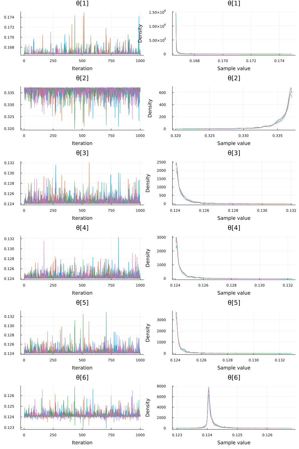
julia> plot(chn)
Note the characteristic “fuzzy caterpillar” look of the trace. This is what you expect to see (and what is absent in the OP, which tells me something is wrong there; I was unable to run your original model, however). A better check is to use ArviZ.plot_rank:
julia> using ArviZ

julia> plot_rank(chn)
Approximately uniform histograms are what you hope to see, and we do.