Hello. Good evening.
I’m doing all exercises of the Sadiku’s book in julia programming.
The code is in github
Im stucked to plot the impulse unit function after get it differentiating the unit step function.
The plot I get is only a line in zero, as plots.jl cant understand that the interval is all zero for values != t0. May someone help?
code:
let
@syms t t₀
u = sympy.Piecewise(
(0, Lt(t, 0)),
(1, Gt(t, 0))
)
@info u
uₜ₀ = subs(u, t=> t - t₀)
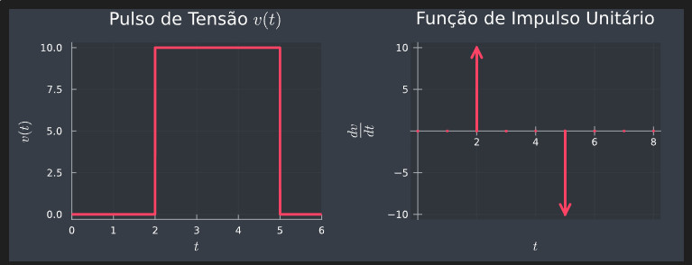
vₜ = 10(subs(uₜ₀, t₀=>2) - subs(uₜ₀, t₀=>5))
@info vₜ
p1 = plot(vₜ, xlims=(0, 6), lw=3, legend=:none, size=(400, 300))
xlabel!(L"t")
ylabel!(L"v(t)")
title!(L"Pulso de Tensão $v(t)$")
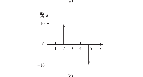
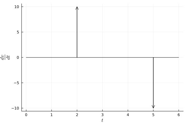
δ = diff(vₜ)
# Ainda não sei como plotar a função de impulso unitário.
@info δ
plot( δ)
end
Results issues
Correct