How to deal with discontinuities in contour plot?

I’m a making a plot of a complex function which has a branch cut discontinuity, and unfortunately it is not easy to parameterize its contour lines, so I rely on calculating the function on the given domain, then taking the contours of the real and imaginary parts, like so:

There is a very clear black contour line which is very rough, due to the discontinuity in the imaginary part of the function, as shown by a heatmap:

My question is: how do I remove this discontinuous curve(or, rather, make it look similar to the others), while mantaining the shape and spacing of all the other ones?

It’s not one thick line, it’s many normal lines very close together, because the contour algorithm encounters this very big step in your data but doesn’t know that there is anything special about it. I’m not sure if there’s a remedy, that’s just how the marching squares algorithm works. Maybe someone else has an idea how this can be improved from the algorithmic side.

Would it be possible to set the grid values to NaN along the branch cut, display the contours and then superpose a thick smooth line to highlight the branch cut location?

Also, could you share the code or equation being plotted?

To remove discontinuity you must use a cyclic colormap, because it is obvious from your posted image that your data for contour plot are periodic. In a cyclic colormap the first rgb color code and the last one should coincide. If they are distinct, depending on values to be colormapped, some artefacts can be displayed.

I suppose I could do that, but I want the contour plot to not show any discontinuities.

I’m plotting the following function, where |z0| < 1:

image

The branch cut happens when the argument of the complex logarithm is a negative real number, where Arg((expression)) goes from -π to π.

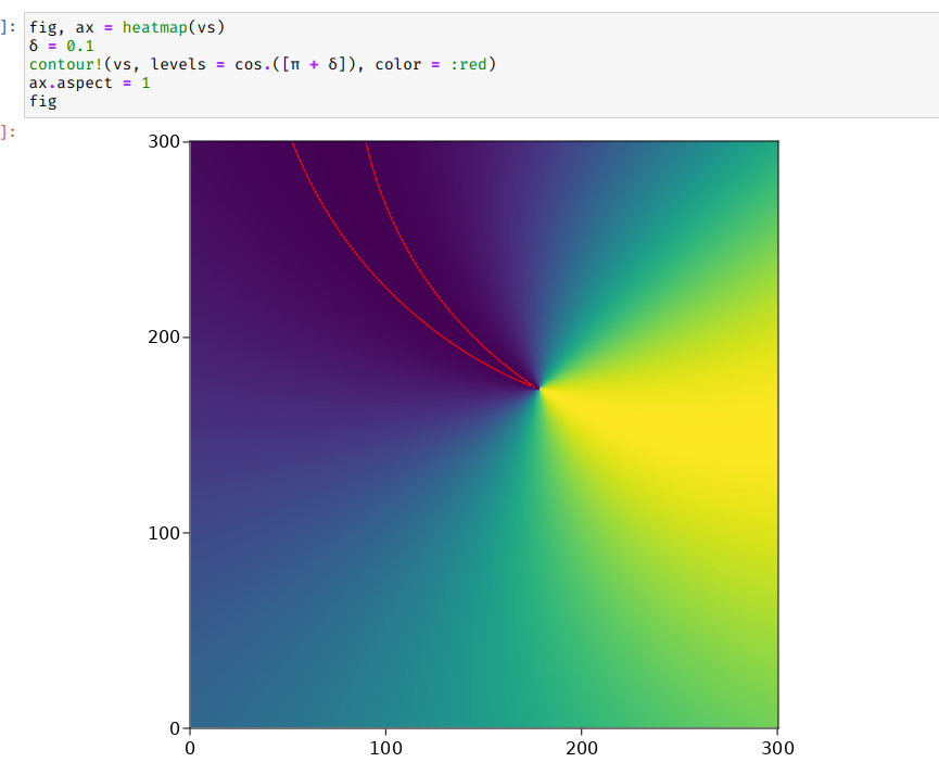
@empet I’m not sure how a cyclic colormap could help. Just to to be clear: I’m not interested in the heatmap, only the contour plot. I’ve also tried applying some periodic function to the imaginary part, such as cos, which maps [-π, π] to a cyclic interval and fixes the problem, but it changes the shape/spacing of the black contours, which is not what I want. Picture for reference:

image

@jules Ah didn’t know that, makes sense. And yeah, I’m also not confident that solely using the contour plot is enough for this, but I’ll look into the marching squares algorithm.

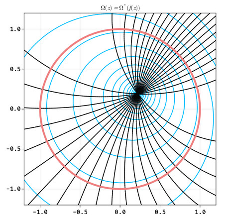
As a side note, I’ve made another plot in which the contour wasn’t the best option, because I was able to parameterize the contour lines and just simply draw them. I tried doing it using the contours, and it turned out OK:

# auxiliary functions
Re(x::Complex) = x.re
Im(x::Complex) = x.im
Re(x::Real) = x
Im(x::Real) = 0
# semi-infinite capacitor
using LambertW
V1 = 10 # Potential of lower plate
V2 = 100 # Potential of higher plate

function g(z::Complex)
    # We need to use different branches of the lambert w function
    k = 0
    if Im(z) > π
        k = 1
    elseif Im(z) < -π
        k = -1
    end
    -lambertw(exp(z-1), k) + z-1
end

Ω(z::Complex) = -im*(V2-V1)/(2π) * z + (V1+V2)/2

fig = Figure(font = "FiraCode Nerd Font")
axis = Axis(fig[1, 1],
    title = L"\Omega(z) = -i \frac{V_2 - V_1}{2 \pi}\left(-W(e^{z-1}) + z-1\right) + \frac{V_1 + V_2}{2}",
    aspect = DataAspect())

xmin, xmax = -5, 10
ymin, ymax = -5, 5

xs = LinRange(xmin, xmax, 100)
ys = LinRange(ymin, ymax, 100)
I  = [Ω(g(x + y*im)) for x in xs, y in ys]
us = Re.(I)
vs = Im.(I)
vs = map(x -> if(isinf(x)) 0 else x end, vs)

contour!(xs, ys, us, levels = 20, linewidth=2, color = :deepskyblue)
contour!(xs, ys, vs, levels = 20, linewidth=2, color = :gray3)
xlims!(low = xmin, high = xmax)
ylims!(low = ymin, high = ymax)
xs = LinRange(xmin, 0, 100)
ys1 = -π*ones(100)
ys2 = π*ones(100)
lines!(xs,ys1, linewidth=8,color = :lightcoral)
lines!(xs,ys2, linewidth=8,color = :lightcoral)

fig

As you can see, no discontinuities, but I had to use different branches of the lambert W function. If I just used the default k = 0 branch:

But, because of the conformal mapping that is used, it is easier to parameterize the function(and as a bonus, we can plot stream arrows):

xmin, xmax = -5, 10
ymin, ymax = -5, 5

umin, umax = -10, 2.2
vmin, vmax = -π, π

# v = A => equipotentials
X(u, v) = 1 + u + exp(u)*cos(v)
Y(u, v) = v + exp(u)*sin(v)

f5 = Figure(font = "FiraCode Nerd Font")
axis = Axis(f5[1, 1],
    title = L"$\Omega(z)$ for a semi-infinite capacitor in 2D",
    aspect = DataAspect())

us = LinRange(umin, umax, 100)
vs = LinRange(vmin, vmax, 100)
vs_arr = LinRange(vmin+0.1, vmax-0.1, 10)

for v in LinRange(vmin, vmax, 30)
    _x(t) = X(t, v)
    _y(t) = Y(t, v)
    lines!(_x.(us),_y.(us), linewidth=2,color = :deepskyblue)
end

for u in LinRange(umin, umax, 30)
    _x(t) = X(u, t)
    _y(t) = Y(u, t)
    
    _xv(t) = -exp(u) * sin(t)
    _yv(t) = 1 + exp(u) * cos(t)
    lines!(_x.(vs),_y.(vs), linewidth=2,color = :gray3)
    arrows!(_x.(vs_arr),_y.(vs_arr), _xv.(vs_arr),_yv.(vs_arr), arrowsize = 10, lengthscale = 0.01)
end

xs = LinRange(xmin, 0, 100)
ys1 = -π*ones(100)
ys2 = π*ones(100)
lines!(xs,ys1, linewidth=8,color = :lightcoral)
lines!(xs,ys2, linewidth=8,color = :lightcoral)

xlims!(low = xmin, high = xmax)
ylims!(low = ymin, high = ymax)

f5

2 Likes

Since you are working with the contour plot of a complex function and you illustrated how irregular is the discontnuity using a sequential colormap, that’s why I suggested to use a cyclic colormap. Cyclic colormaps are used in the so called domain coloring representation of a complex function.
If a function f(z) is defined on a (rectangular) region in the complex plane, then the argument of f(z) is plotted as a heatmap on that region, while over heatmap are displayed the contour lines of the modulus |f(z)|.

The argument of log(z):
logz
argument and log modulus:
rsz_logz-contours

Thanks for the reply! Yes, domain coloring is interesting, but not what I’m looking for. I specifically want to “patch up” the discontinuity in the contour plot.

I think you’re almost there with this approach: now, instead of asking for contour values equidistantly spaced in the mapped (i.e., under cos) space, just request contour values that are equidistantly spaced in the original space by asking for specific contour values (e.g. cos(range(0, 2*pi))).

1 Like

Thanks! That solves the problem of the shape, but it still doesn’t provide the “best” result. The algorithm still seems to have trouble detecting the contour line at cos = -1 and cos = 1:

I’ve also plotted the heatmap of the cos function with contour lines:

(As you can see, there’s always gaps where arg(z) would be discontinuous, and also where arg(z) ≈ 0, curiously enough)

For reference, I used levels = cos.(LinRange(0, π, 15)) for those plots, which provides the best results so far, but also experimented with a range of (0, 2π) as you said, and many other ranges.

I’m also using a grid Size of 300×300. Increasing the resolution definitely increases the quality of the contours with this hack, but then I’m not sure it is even worth it, because the contours already look pretty good without any cos/sin/whatever mapping. 3000×3000 plot for reference(without any transformations):

My problem with this “just increase grid size!” solution is that it’s reeeally slow, and I need to create these plots for animations.

Edit: I think I may have found the reason as to why the contour algorithm has trouble with the iso-lines cos = 1 and cos = -1. By plotting a single contour level, we see that the two opposing sides of the discontinuity are considered to have the same value(which is not surprising, because they do)

This happens for any value of δ. The problem is that, as δ goes to zero, these two parts of the contour get fuzzy and stop behaving as we’d expect:

The same happens for δ around 0:

Which is why we see no contours for cos = ±1

The problem is that you are asking for contour lines exactly at the minimum/maximum of a function (e.g. marching cubes/squares will want to “box-in” the contour value which is not possible if there’s no higher/lower value).

To fix it, you could just move the problematic maxima/minima to a contour value you’re not looking at e.g. by changing your mapping function from cos(Arg(z)) to cos(Arg(z)+phi). You could e.g. choose phi = 2*pi/N where N denotes your desired number of contour values. If you apply the map to both data and contour values it won’t change the appearance of your graph.

3 Likes

Ah I see, didn’t know that about the marching squares algorithm! Thanks!

I’ve now re-implemented the plot with an offset δ, and the animation looks better(just need to improve the stability of the blue contours):

output2

For reference, I modified your idea of using phi slightly to just shortening the range of desired contour values by δ, effectively not requesting contours to be drawn at the max/min value, as you suggested. The code for the animation is below for reference:

Re(x::Complex) = x.re
Im(x::Complex) = x.im
Re(x::Real) = x
Im(x::Real) = 0

Q = 1.0
z0 = 0.5 + 0im

f(z) = im*(1+z)/(1-z)
w0 = f(z0)

Ω(w::Complex, w0::Complex = w0) = log((w - w0)/(w - conj(w0))) #*Q/2π not necessary for contours

xmin, xmax = -1.2, 1.2
ymin, ymax = -1.2, 1.2

xs = LinRange(xmin, xmax, 100)
ys = LinRange(ymin, ymax, 100)

# Path for w0 - lemniscate
λ(t, a) = a*√2*cos(t)*(1 + sin(t)*im)/(1+sin(t)^2)

# Define fig, axis
fig = Figure(font = "FiraCode Nerd Font")
axis = Axis(fig[1, 1],
    title = L"$\Omega(z) = Ω^*(f(z))$",
    aspect = 1)
## Definitions for animation
time = Node(0.0)
t_iterator = range(0, 2π, length=10*60)
#filter inf
function rm_inf(z)
    if isinf(z)
        0
    else
        z
    end
end
##
δ = 0.1
I(t)  = [rm_inf(Ω(f(x + y*im), f(λ(t, 0.5)))) for x in xs, y in ys]
us = @lift Re.(I($time))
vs = @lift cos.(Im.(I($time)))

# Main plot
contour!(xs, ys, us, levels = 20, linewidth=2, color = :deepskyblue)
contour!(xs, ys, vs, levels = cos.(LinRange(δ, π-δ, 12)), linewidth=2, color = :gray3)
# Plot red circle ∂D
ts = LinRange(0, 2π, 100)
gamma(t) = (cos(t), sin(t))
lines!(gamma.(ts), linewidth = 5, color=:lightcoral)

# Configs
xlims!(low = xmin, high = xmax)
ylims!(low = ymin, high = ymax)

record(fig,joinpath(@__DIR__, "videos", "anim.mp4"), t_iterator;
           framerate = 60) do t
       time[] = t
end

Edit: Also using @tchr 's ideas, the instability in the blue contours in the frame-by-frame iteration is caused by the fact that the option levels = 20 accounts for levels ranging from the minimum to the maximum value of Ω in the domain(which, of course, changes as we change z0). The fix is quite easy, then: just provide a LinRange in which we have fixed values for the contours. The following animation uses levels = LinRange(-3, 1, 20), for example: Imgur: The magic of the Internet

3 Likes

Is this the new Dr Who title sequence?

1 Like