So, if we given these two input to a function, I need to calculate the nearest point on that line. As shown in the following picture, Black dots shows the line input and orange dot shows the expected output from the function.
Parse your input to get a list of line segments (\vec{s}_i, \vec{t}_i).
Project your point \vec{p} onto each line segment to get \vec{q}_i:
Let \vec{v}_i = \vec{t}_i - \vec{s}_i and \vec{p}_i = \vec{p} - \vec{s}_i. Then \vec{s}_i + t \vec{v}_i, where t = \frac{\vec{v}^T \vec{p}_i}{\vec{v}_i^T \vec{v}_i}, is the orthogonal projection onto line(\vec{s}_i, \vec{t}_i). You are interested in line segments, so we need to clamp the parameter t. So, \vec{q}_i = \vec{s}_i + \min(1, \max(0, t)) \vec{v}_i.
Use \vec{q}_i with the minimum distance d_i from \vec{p}:
You can use the squared euclidean distance, which is simply a dot product: d_i = (\vec{p} - \vec{q}_i)^T (\vec{p} - \vec{q}_i).
In julia, the second point can be implemented like this
using LinearAlgebra
# given a point `p` and a line segment starting at point `s` and ending at point `t`,
# find a point on that line that is closest to `p`
function nearest_point_on_line(p, s, t)
    @assert ndim(s) == ndim(t) == ndim(p)
    v = (t - s)
    t = clamp((v ⋅ (p - s)) / (v ⋅ v), 0, 1)
    return s + t * v
end
Amazing @visr , You’re a lifesaver. This is exactly what I needed.
Just a small question along the same, Since these line strings are on the earth’s surface, how would it affect the accuracy of the returning on_linestring value?
The problem of the GEOS solution is … it’s not correct because GEOS is a Cartesian library. When working with geographical coordinates you want the point to be along a great circle. In this case the difference is small, but it is no zero. GMT computes it though I find some issues that need to be ironed up. Namely, to compute this one need to save the lines segments in a file first
Oh nice @joa-quim , This is exactly what I needed. Appreciate the help mate. Just wondering are you by any chance familiar with this error ? I’m using Mac with M1 processor.
Failed to precompile GMT [5752ebe1-31b9-557e-87aa-f909b540aa54] to /Users/cbandara/.julia/compiled/v1.6/GMT/jl_rcWYt7.
ERROR: LoadError: SystemError: opening file “/Users/cbandara/.julia/packages/GMT/1kBBX/deps/deps.jl”: No such file or directory
When I tried to install this libaray, it keeps giving me this error. I’m using Mac with M1 processor.
Btw, by any chance are you familiar with this error ? I got this when I try to add the library ?
Failed to precompile GMT [5752ebe1-31b9-557e-87aa-f909b540aa54] to /Users/cbandara/.julia/compiled/v1.6/GMT/jl_rcWYt7.
ERROR: LoadError: SystemError: opening file “/Users/cbandara/.julia/packages/GMT/1kBBX/deps/deps.jl”: No such file or directory
Hmm, that file (deps.jl) is generated by the build process. Don’t know why it was not in your case.
Try to run import Pkg; Pkg.build("GMT"). If it doesn’t solve it better to move this into a GMT.jl issue
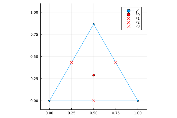
There is the issue of multiple results with the same (or almost the same distance). Perhaps an eps parameter will help to determine closest points, and a vector/set returned. Or a findfirst logic, or return the closest point and the gap to the next closest point.
The simplest example to think of is the middle of an equilatral triangle.
To output multiple nearest points within a specified tolerance:
Code
# Assumes that the input line nodes are spatially ordered

distance(P1, P2) = hypot(P1[1] - P2[1], P1[2] - P2[2])

dot(x,y) = sum(a*b for (a,b) in zip(x,y))

# Adapted from @barucden
# Given a line segment starting at point S[1] and ending at point S[2],
# find a point on that line that is closest to P0
function nearest_point_on_segment(S, P0)
    V = S[2] - S[1]
    t = clamp(dot(V, P0 - S[1]) / dot(V, V), 0., 1.)
    return S[1] + t * V
end

# Input data
P = [ [0.0, 0.0], [1.0, 0.0], [0.5, sqrt(3)/2], [0.0, 0.0] ]
P0 =  [0.5, sqrt(3)/6]

# Find the closest points on each of the segments
S = [ [P[i], P[i+1]] for i in 1:length(P)-1]
Pn = nearest_point_on_segment.(S, Ref(P0))
d = distance.(Pn, Ref(P0))
dmin = minimum(d)
ϵ = 1e-3 * dmin   # tolerance on distance
ix = findall(x -> abs(x - dmin) < ϵ, d)

# Plot results
using Plots
p = plot(first.(P), last.(P), m=:o, ms=3, ratio=1, lims=(-0.1,1.1))
scatter!((P0[1], P0[2]), c=:red, label="P0")
for i in ix; scatter!((Pn[i][1], Pn[i][2]), c=:red, m=:x, label="P$i"); end
p
@Dan Ahh, Yes that makes sense. This is the issue with LibGEOS library, based on the answer provided by @visr , does that mean on_linestring can have multiple values when the line string is almost a triangle?
@Chamika_Kasun if you ever feel the need to modify these algorithms or use a different combination of functions without reaching out to external libraries not written in Julia, consider reading the source code of Meshes.jl.
Regarding distance calculations, we plan to add more methods here after we finish the implementation of a related set of features. Regarding nearest neighbors, take a look at the examples here.