function Π(E,W)
    E = 1:10
    W = 1:10
    sqrt(E)+4*W
end
When I try to enter this function, it gives me Π as an output, and If if I try to use Π as a function, I’m told that I don’t get a function.
function Π(E,W)
E = 1:10
W = 1:10
sqrt(E)+4*W
end
When I try to enter this function, it gives me Π as an output, and If if I try to use Π as a function, I’m told that I don’t get a function.
What do you mean by “When I try to enter this function”? Are you writing it in the REPL? or is it in a script that you run with include? Pasting your code into the repl successfully defines a function for me. If you’re writing that in a script maybe there’s something funny with the unicode support in your text editor? That’s just a guess.
As a side note that you may already be aware of, your function doesn’t actually use the input arguments E and W. It redefines those variable names inside the function. Also, you can’t take the sqrt of a range. You need to do
sqrt.(E) + 4*W
I’ll change the material, I’m trying to figure out plots. I want to plot sqrt(x) + z as parell curves.
please produce a MWE with error messages so we can help you
OK, let me try to decrypt the message ![]()
When I try to enter this function, it gives me Π as an output,
I think what you mean is “When I type or copy paste this funcion to the terminal, it returns Π”.
Yes, that’s true. If you enter something into the REPL (the “interactive Julia terminal”), it will show the representation of the last expression or the return value itself. In this case, the function is showed as “Π (generic function with 1 method)”.
That’s perfectly fine, nothing wrong here.
julia> function Π(E,W)
           E = 1:10
           W = 1:10
           sqrt(E)+4*W
       end
Π (generic function with 1 method)
The next one is a bit confusing:
If if I try to use Π as a function, I’m told that I don’t get a function.
I think you just tried to execute the function with some parameters (I just put in 1 and 2, as it doesn’t matter since you are ignoring those):
julia> Π(1, 2)
ERROR: MethodError: no method matching sqrt(::UnitRange{Int64})
Closest candidates are:
  sqrt(::Float16) at math.jl:1019
  sqrt(::Complex{Float16}) at math.jl:1020
  sqrt(::Missing) at math.jl:1072
  ...
Stacktrace:
 [1] Π(::Int64, ::Int64) at ./REPL[1]:4
 [2] top-level scope at REPL[2]:1
What you see is an ERROR. Nobody “tells you” that you “don’t get a function”. It’s just the fact that the sqrt function has no method which takes a UnitRange{Int64}.
The way you describe your problem makes me think that you have almost no idea about how programming languages work, so I’d recommend to read some introductory material: Get started with Julia
On the other hand, I’d like to show you want you wanted to do, although it will only solve a tiny part of the main problem (which is: you need to invest time to learn coding).
julia> function Π(E, W)
           sqrt.(collect(E)) .+ 4*collect(W)
       end
Π (generic function with 1 method)

julia> Π(1:10, 1:10)
10-element Array{Float64,1}:
  5.0
  9.414213562373096
 13.732050807568877
 18.0
 22.23606797749979
 26.44948974278318
 30.64575131106459
 34.82842712474619
 39.0
 43.16227766016838
I however don’t know what you want to plot here.
Try
using Plots

Π(E,W) = sqrt(E)+4*W
E = 1:10
W = 1:10

contour(E,W,Π)
And as tamasgal said,
Last but not least: Please read: make it easier to help you - #8
![]()
Ah yeah, that might be the original problem ![]()
Been trying to do other stuff as a go along, but studying programming is a good idea. I’m trying to plot curve E,W, on plane Π
What does that mean? Can you draw a figure with something resembling what you want to plot? What’s the code to do it in any other programming language?
I’d like to plot a curve of U.
It’s not clear to me what you want to plot, but consider the following:
Π = (e,w) -> sqrt(e) + 4w
Some possibilities (assuming you have issued the command using Plots…):
plot(1:10,1:10,Π,st=:surface)
gives:
st is short for seriestype], while
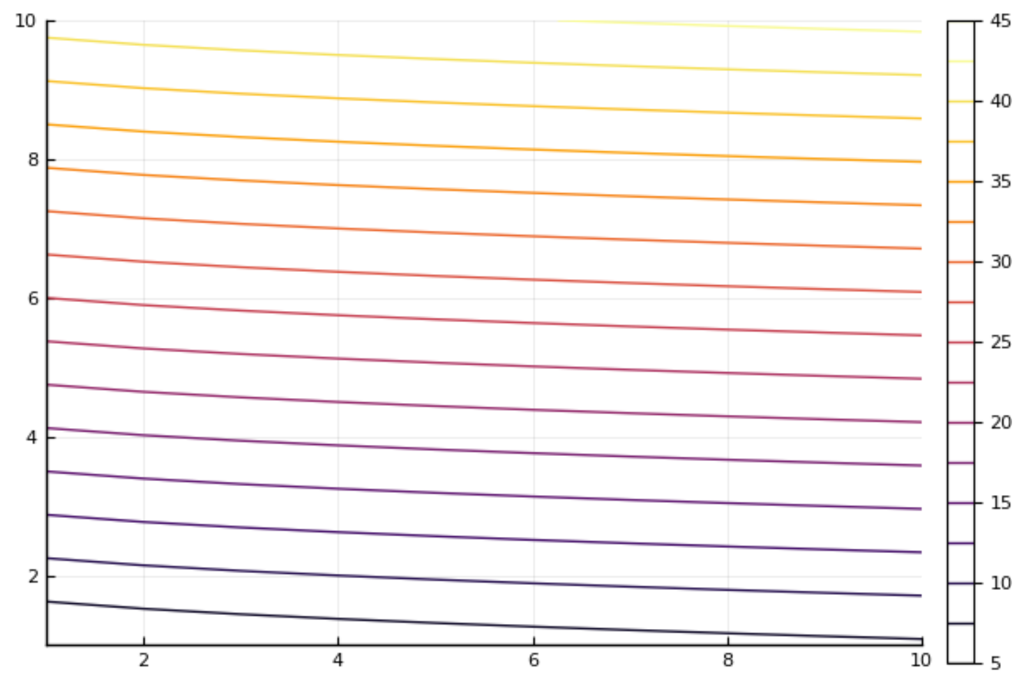
plot(1:10,1:10,Π,st=:contour)
gives:
plot()
for w in 1:10
    e = 1:10
    plot!(e,Π.(e,w),label="")
end
plot!()
[the default seriestype is st=:path] gives:
perfect!
What if I wanted to add another function to the same chart?
A little more fun function:
f = (x,y) -> sin(x)*cos(y)
Plotting it in 3D:
x = range(-pi,pi,length=100)
y = range(-pi,pi,length=100)
plot(x,y,f,st=:surface)
gives:
plot(x,y,f,st=:contour)
plot!(x,x->0.25x^2,lw=2.5,lc=:black)
gives:
p1 = plot(x,y,f,st=:surface)
p2 = plot(x,y,f,st=:contour)
plot(p1,p2,layout=(1,2),size=(800,400))
U(E,W)= E*W #Utility function
E = 0:40
W = 10:100
plot(0:40,10:100,Π,st=:contour)

B(E,W)= (40-E)/W # budget line function
E = 0:40
plot(0:40,10:100,B,st=:contour)

plot(0:40,10:100,U,st=:contour) #Plot{Plots.GRBackend() n=1}
plot!(0:40,10:100,B,st=:contour) #Plot{Plots.GRBackend() n=2}
No errors, but does not produce an overlapping graph. Is that because
plot(x,y,f,st=:contour)
plot!(x,x->0.25x^2,lw=2.5,lc=:black)
combines a 2d and a 3d graph?
Combining contours has limitations. Only the most recent plot contours match the colorbar, and there is only one z-scale. So, must scale your contours to equal z-range (you see where I used the factor 1500).
using Plots

U(E,W)= E*W #Utility function
B(E,W)= (40-E)/W # budget line function

X,Y = 0:0.5:40, 10:0.5:100
plot(X,Y,(x,y)->1500*B(x,y),st=:contour, dpi=200,color=:red, contour_labels = true, linewidth=2)
plot!(X,Y,(x,y)->U(x,y),st=:contour, levels=20, linewidth=2)
plot!(X,x->0.05x^2,lw=6.0,lc=:green, xlims=extrema(X), ylims=extrema(Y), alpha=0.5)
In PyPlot, it is possible to insert contours in 3D plots, and decide the vertical position z. I sometimes miss that in Plots.
For somebody new it can be confusing to see that collect is needed here:
but not here:
o here:
It’s not needed here. But the broadcasting is. Broadcasting works just fine on generators or ranges.
Maybe I should be doing Python first, I have a mixed knowledge of R and Julia, was going to just study programming after I finish studying Economics for the summer.