Essay: Julia and Projective Geometric Algebra

There appears to be a lot of overlap in the fields of science interested in Julia and the fields of science interested in geometric algebra. Perhaps the two communities would benefit from each other?

In an attempt to encourage that interaction from the Julia side, I have posted an essay Julia and Projective Geometric Algebra that gives an introduction to projective geometric algebra and a Julia port of bivector.net’s C++ reference implementation of 3D projective geometric algebra in the essay’s appendix. All of the Julia code in that essay is currently just an early draft but when I complete the second example application I’ll put all the code in a github public repository.

29 Likes

The essay now includes the projective geometric algebra code for the Julia and Makie implementation of the following inverse kinematics and 3D slicing example applications:

ikv
tslice

Following my interests, I plan to extend the inverse kinematics example with self-collision avoidance and I plan to generalize the 3D slicer example so that it slices a 5002 triangle face model of a chocolate bunny. However, the purpose of the essay is to spark interest in the Julia community. Are there a couple other Steven De Keninck example applications of projective geometric algebra that are especially interesting to the Julia community? (Because projective geometric algebra is still quite new to me, I for now will stay within the safe confines of Steven De Keninck’s many example applications.)

Based upon which example application links get followed the most, I’ll attempt to include the two most popular example applications in the essay. Here are some example application options but I am open to others:

19 Likes

polyx

The essay now includes a Julia and Makie implementation of a polygon intersection testing example application. I think the highlight of the application is how the following Makie code generates the 15 second .mp4 video (later converted into a repeating animated .gif) in just 3.1 seconds (on my laptop computer).

	# record spinning polynomial following path
	record(fig, "polyx.mp4", 1:nFrame) do iFrame
		ROT = [cos(THETAS[iFrame]) -sin(THETAS[iFrame]);
			   sin(THETAS[iFrame])  cos(THETAS[iFrame])]
		nPartition = length(B)
		for iPartition = 1:nPartition
			MB[iPartition] = Float32.((ROT * B[iPartition]) 
				.+ PATH[:,iFrame])
			OBS_C[iPartition][] = (sat(A, MB[iPartition]) == 0) ?
				RGBA(1, 0, 0, 0.5) : RGBA(0, 1, 0, 0.5)
			OBS_MB[iPartition][] = MB[iPartition]
		end # for each partition
	end # for each video frame

The geometry in this 2D application is simple enough that PGA didn’t seem helpful. However, given that polygon intersection testing was the most requested PGA example application, I’ll include both a PGA version and a non-PGA version in the essay. (Perhaps the comparison will be helpful.)

7 Likes
julia> include("ripga2d.jl")
utest (generic function with 4 methods)

julia> P = point(2,3); println(toStr(P) * ": $P")
3*e01 + 2*e20 + e12: Float32[0.0, 0.0, 0.0, 0.0, 3.0, 2.0, 1.0, 0.0]

I’ve ported bivector.net’s pga3d.cpp (a C++ reference implementation of 3D PGA) to Julia and Julia’s REPL is now capable of evaluating PGA expressions that include variables and functions, which is particularly useful when exploring PGA concepts and debugging PGA applications.

For example, the essay’s first section (Why Projective Geometric Algebra?) now includes a narrated REPL session that introduces three PGA superpowers:

  • defining variables clearly,
  • offering a dual approach to thinking about geometry, and
  • staying “above the fray” of special cases.
3 Likes

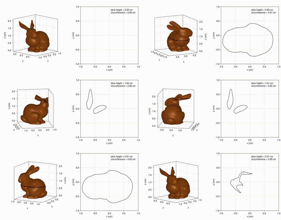
sl

This animation of 3D slicing was generated by the following setup of GLMakie observables:

	# initialize figures
	fig = Figure(resolution = (1000, 500))
	ax3d = Axis3(fig[1,1],
		elevation = pi/16,
		azimuth = -5*pi/8,
		viewmode = :fit,
		zlabel =   "z (cm)",
		aspect = (1,1,1))
	m = mesh!(ax3d, normal_mesh(F),
		color = :chocolate4,
		shading = true)
	ax2d = Axis(fig[1,2],
		limits = (-1,1, -1,1),
		xlabel = "x (cm)",
		ylabel = "y (cm)")

	# plot initial observable data
	SEG = fill(NaN32, 3, 3*nF) # line SEGment buffer
	MEASURE = zeros(Float32, 2)
	zCut::Float32 = 1f0
	nCol = zslice(zCut, F, TZ, TI, SEG, MEASURE)
	SEG_obs = Observable(SEG)
	slice2d = @lift @view $SEG_obs[1:2,1:nCol]
	slice3d = @lift @view $SEG_obs[:,1:nCol]
	strHeight = @sprintf( 
	       "slice height = %.2f cm\ncircumference = %.2f cm",
		zCut, MEASURE[1])
	str_obs = Observable(strHeight)
	lines!(ax3d, slice3d,
		linewidth = 5,
		color = :black)
	lines!(ax2d, slice2d,
		color = :black)
	text!(ax2d, str_obs,
		position = (0.05, 0.75),
		space = :data)
	fig
	
	# generate video of slicing
	zMax = 2.0
	nFrame = 720
	record(fig, "sl.mp4", 1:nFrame) do iFrame
		ax3d.azimuth[] = -3pi/4 - 2pi*(iFrame-1)/nFrame
		zCut = zMax - abs(zMax - 2*zMax*(iFrame-1)/nFrame)
		nCol = zslice(zCut, F, TZ, TI, SEG, MEASURE)
		notify(SEG_obs)
		str_obs[] = @sprintf(
		       "slice height = %.2f cm\ncircumference = %.2f cm", 
			zCut, MEASURE[1])
	end # for each video frame

The essay now includes that fast 3D slicing example application without PGA. On my laptop computer Makie generates the above 30 second video in 8.2 seconds. I haven’t yet finished the PGA version but I suspect it will be about the same speed, like the other 2D and 3D geometry applications I’ve ported from ganja.js to Julia and Makie.

In dimensions higher than 3D, it is easy to see the advantages of PGA but I haven’t yet encountered a 2D or 3D geometry application that gets faster or simpler using PGA. However, in his demonstration of his origami example application, Steven De Keninck suggests that PGA makes that 3D geometry application “a lot more fun and a lot more easy”, so I am inclined to try porting that ganja.js origami application next.

5 Likes

After several false starts, I think I stumbled upon a good approach to introducing Projective Geometric Algebra to Julia programmers: a “REPL sandwich” that uses a REPL session to introduce a couple PGA concepts followed by an extension of those concepts into an example application followed by a REPL session that highlights key concepts from that example application. For example, the essay now includes a “REPL sandwich” that

  • starts with a REPL session introducing a couple 3D PGA concepts to calculate the intersection of a triangle and a plane,
  • extends those concepts to implement a 3D slicer application (e.g., for 3D printing), and
  • ends with a REPL session (listed below) highlighting PGA’s ability to efficiently calculate the area of an arbitrary polygon by summing its edges. Specifically, the REPL session estimates the area of the unit circle by summing the edges of a polygon that approximates the shape of the circle.

If the idea of calculating the area of a polygon by summing its edges prompts you to start reconsidering your mental model of integration, welcome to PGA and don’t worry about it. Confusion is common. I think the source of my PGA confusion is probably that I don’t yet fully grasp PGA duality. Steven De Keninck jokes that the way to know you have achieved an understanding of PGA duality is when your mind is blown twice.

julia> include("ripga3d.jl");

julia> r = 1.0;

julia> nTheta = 128;

julia> THETA = LinRange(0,2*pi,nTheta+1);

julia> VC = Float32.([ # Vertex Coordinates
           r .* cos.(THETA');
           r .* sin.(THETA');
           zeros(1,nTheta+1)]);

julia> V = point(VC); # Vertex PGA expressions

julia> E = V[:,1:nTheta] & V[:,2:nTheta+1]; # Edges (CCW)

julia> area = normIdeal(sum(E, dims=2)[:]) / 2
3.1403282f0
2 Likes

polyx3

In example 3.3, the essay now includes a 3D polygon intersection testing example. The moving cube turns green only when the separating axis test (SAT) detects a separating plane between the cubes, meaning they are not intersecting. (On my laptop computer, Julia and GLMakie generated the 15 second .mp4 video in 3.9 seconds.)

The “REPL sandwich” framework is helpful with this example because the first REPL session introduces the simplest form of the inner product (the fundamental operation in the separating axis test) and the last REPL session shows that for the 3D inner product (or any dimension > 2) of two lines in a plane must also specify the plane in order for the orientation of the inner product result to be correct.

5 Likes

origami

The bivector.net ganja.js origami application example is now ported to Julia and GLMakie in example 3.4 of the Julia and Projective Geometric Algebra essay. (On my laptop computer, Julia and GLMakie generated the 66 second .mp4 video in 10.3 seconds.)

The example’s “REPL sandwich” starts with the following REPL session demonstrating the application’s fundamental rotation operation and that the direction of rotation depends upon the orientation of the rotor’s pivot line.

julia> include("ripga3d.jl"); # REPL 1 origami

julia> P = point(Float32.([ # PGA points
           0 0 1;
           0 0 0;
           0 1 0]));

julia> PL = P[:,1] & P[:,2]; # Pivot Line

julia> R = rotor(pi/2, PL);

julia> result = toCoord(R >>> P[:,3])
3-element Vector{Float32}:
 0.0
 0.99999994
 0.0

julia> PL2 = P[:,2] & P[:,1]; # Pivot Line 2

julia> R2 = rotor(pi/2, PL2); # Rotor 2

julia> result2 = toCoord(R2 >>> P[:,3])
3-element Vector{Float32}:
  0.0
 -0.99999994

A common argument against using PGA is that it inefficiently takes 16 floats to store a 3D point instead of just three. However in many PGA applications, only a small portion of the 3D points are converted to PGA points at any one time. For example in this origami application, all the vertices are stored in a Makie mesh and only the vertices in that mesh currently being rotated during a fold are temporarily converted to PGA points. Therefore the second REPL session in the origami example’s REPL sandwich shows how to construct a Makie mesh directly from 3D points (e.g., after being rotated using PGA).

julia> include("ripga3d.jl"); # REPL 2 origami

julia> using GLMakie;

julia> using GeometryBasics;

julia> PC = Float32.([ # Point Coordinates
           0 0 1;
           0 0 0;
           0 1 0]);

julia> V = Point{3, Float32}[]; # mesh Vertices

julia> push!(V,PC[:,1]); push!(V,PC[:,2]); push!(V,PC[:,3]);

julia> F = TriangleFace{Int64}[]; # mesh Faces

julia> push!(F,[1,2,3]);

julia> result = GeometryBasics.Mesh(V,F)
Mesh{3, Float32, Triangle}:
 Triangle(Float32[0.0, 0.0, 0.0], Float32[0.0, 0.0, 1.0], Float32[1.0, 0.0, 0.0])
6 Likes

fabrik2dv16

As a proof of concept, I’ve added self-collision avoidance by slightly nudging the pivot points before each first relaxation pass in the FABRIK inverse kinematics algorithm. Given the resemblance to double pendulums, it is not surprising that the FABRIK algorithm is extremely sensitive to initial conditions and can avoid collisions with tiny initial nudges. In the animation, when the collision avoidance nudge “pressure” is zero the typical FABRIK algorithm has no self-collision avoidance but when the collision avoidance nudge “pressure” is 0.001 there is a single point source of low pressure air at the center of the elliptical path blowing out the robot’s pivot points enough to avoid self-collisions. The PGA code is in example 3.1 of the Julia and Projective Geometric Algebra essay.

6 Likes

tetra3x

I’ve updated the essay because what I previously thought was a magical PGA formula for calculating the volume of a triangle mesh turned out to be no more magical than calculating the volume of a parallelepiped, which can also be done with linear algebra determinants.

Still learning about geometry, I did not see why a parallelepiped’s volume is exactly six times the volume of any of its corner tetrahedra until I implemented the following animation:

# tetra3x.jl : show tetrahedron volume is 1/6 parallelepiped volume
#= tetrahedron 1 (tetra1.obj)
v -1 -0.5 0
v -1 -0.5 1
v  1 -0.5 0
v -1  0.5 0
f 1 4 3
f 1 3 2
f 1 2 4
f 2 3 4
=#
#= tetrahedron 2 (tetra2.obj)
v -1 -0.5 1
v  1 -0.5 0
v  1 -0.5 1
v -1  0.5 0
f 1 2 3
f 4 1 3
f 4 3 2
f 4 2 1
=#
#= tetrahedron 3 (tetra3.obj)
v -1 -0.5 1
v  1 -0.5 1
v -1  0.5 0
v -1  0.5 1
f 1 4 3
f 2 4 1
f 2 3 4
f 2 1 3
=#

using GLMakie, GLMakie.FileIO
using Images # for RGBA
include("ripga3d.jl") # needed for satpga() not sat()

# partition tetrahedron
function tetra3x()

	# initialize figure
	fig = Figure(size = (800, 800))
	ax3d = GLMakie.Axis3(fig[1,1],
		elevation = pi/8,
		azimuth = -pi/4,
		viewmode = :fit,
		aspect = (1,1,1),
		limits = (-2.,2., -2.,2., -2.,2.),
		titlesize = 28,
		title = "partition of half parallelepiped into three tetrahedra")
	
	# load meshes of three tetrahedra
	T1 = load("tetra1.obj")		# tetrahedron 1 (stationary)
	T1C_obs = Observable(RGBA(1, 0, 0, 0.5))
	T2 = load("tetra2.obj")
	T2C_obs = Observable(RGBA(0, 1, 0, 0.5))
	T3 = load("tetra3.obj")
	T3C_obs = Observable(RGBA(0, 0, 1, 0.5))

	# initialize plot containing observable data
	mesh!(ax3d, T1, color = T1C_obs)
	mesh!(ax3d, T2, color = T2C_obs)
	mesh!(ax3d, T3, color = T3C_obs)
	fig
	
	# generate video
	iState = 0
	nFrame = 360
	record(fig, "tetra3x.mp4", 1:nFrame) do iFrame
		if mod(iFrame-1, 60) == 0
			iState += 1
			if iState == 4
				T1C_obs[] = RGBA(1, 0, 0, 0)
			elseif iState == 5
				T1C_obs[] = RGBA(1, 0, 0, 0.5)
				T2C_obs[] = RGBA(0, 1, 0, 0)
			elseif iState == 6
				T2C_obs[] = RGBA(0, 1, 0, 0.5)
				T3C_obs[] = RGBA(0, 0, 1, 0)
			end
		end
		ax3d.azimuth[] = -3pi/4 - 2pi*(iFrame-1)/nFrame
	end # for each video frame
end # tetra3x()

# quick and dirty ffmpeg conversion from tetra3x.mp4 to tetra3x.gif:
# /tool/ffmpeg-2022-07/bin/ffmpeg.exe -i tetra3x.mp4 -r 24 -s 480x480 -loop 0 tetra3x.gif

4 Likes