Not a specific question about julia, but I’m sure someone can help me get a correct idea about the following problem.
I know that the average tax applied in the various US states on the price of cigarettes is mu=73cents, while the standard deviation is sigma=48cents.
Can one argue on the basis of this information that the distribution has a bell shape?
no. The existence of a mean and standard deviation doesn’t imply much about the shape (it only really implies an upper bounds on how heavy the tails are).
Also, there are 50 states exactly, so the actual distribution is 50 point masses.
The data behind these numbers is the tax in each state. If we write the tax rates as x_i where 1 <= i <= 50 (supposiing there are 50 states). What the OP says amounts to the following two constraints: \sum_{i=1}^{50} x_i = 50*73 \sum_{i=1}^{50} x_i^2 = 50*(73^2+48^2)
where the units are cent in first equation and cent^2 for the second equation.
This has 50 unknowns with two equations, and that’s most of what the data guarantees.
(*) the second equation assumes an un-corrected std-dev calculation.
The answer just illustrates how little the mean and std-dev constrain the data, and any conclusion would need more input from common sense. For example, one might assume no state subsidizes smoking and therefore x_i >= 0 for all i.
One thing you could do is leverage the central limit theorem and argue that the tax is the sum of many random factors, such as demographics and values of people in different states, legislative process, etc. Of course, it may not be a very strong argument, but it might be plausible.
This was one of the reflections I made (the problem was posed to me by my daughter who studies psychology.) but I would like to see it developed with some formalism that perhaps would help me understand better
Those 50 states would probably have a few states with a round number for a tax, say 50c or 0c. Even if a few states have the same tax, it makes a model with an underlying single distribution for all states, which is unimodal (i.e. bell-like shaped) statistically significantly unlikely.
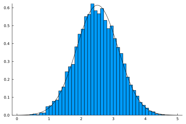
For a formal treatment, I recommend researching the central limit theorem and the Berry-Esseen theorem, which discusses convergence to a normal distribution under stronger assumptions. If a demonstration will suffice, you can do something like the following:
using Plots

using Distributions

using Random

Random.seed!(90)

n_vars = 5

n_samples = 10_000

samples = rand(n_samples, n_vars)

sums = sum(samples, dims=2)

histogram(sums, norm=true)

x = range(0, 5, length=100)

dens = pdf.(Normal(mean(sums), std(sums)), x)

plot!(x, dens, leg=false, grid=false, color=:black)
I’m sure the psychology students will be delighted to learn about this theorem and all the conditions and history of the central limit theorem. Especially going over the several right (and wrong) proofs in history
I would have thought the random factors boils down to the two polarized political parties (not so random in a continuous spectrum)
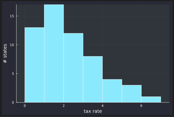
just out of curiosity, went searching for the tax stats online, you can almost tell the political party of the state by looking at the tax. (suggest strong correlation in the sample data, and CLT assume independent data?)
With the following data you get almost the same values as the example on which the question is asked.
In some cases the sale of cigarettes is subsidized. What political party would this be in the USA ?
How does the histogram function work?
How do you use 10000 values?
I did not go through it in sufficient detail to understand what weak dependence means. My guess is that convergence will take longer with correlated random variables. If they are maximally correlated, the CLT will not apply.