[ANN] SymbolicApproximators.jl: methods for symbolic time series discretization

Announcing SymbolicApproximators.jl, a Julia package implementing Symbolic Aggregate approXimation (SAX) and related methods for symbolic discretization and dimension reduction. These techniques allow you to take continuous-valued sequences (including but not necessarily limited to time series) and then use things like string algorithms and machine learning algorithms for categorical data.

(Note: it has a couple hours left before registration completes so you will not be able to install it just yet from the General Registry.)

So far I’ve only implemented a few algorithms. More will follow soon. I’ve aimed for this to be the fastest implementation of SAX and SAX-family algorithms available, and some informal tests so far have shown that it may be. Basic usage of SAX seems to be about 8x faster than in R’s jmotif package, and > 3000x faster than Python’s saxpy.

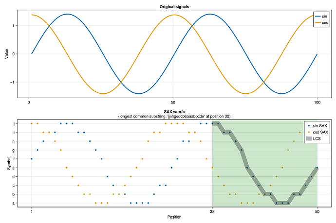
Here’s a quick demo. (See here for the full code.) If we have two continuous signals, let’s say a sine wave and a cosine wave, we can use this package to:

  • convert them to reduced-size discrete representations
    • specifically here we’ll use the symbols a through j and a “word” size of 50
  • we’ll pass those time series into a suffix automaton structure, with which we can compute the longest common substring (lcs) between the reduced time series
using SymbolicApproximators
using SuffixAutomata
using StatsBase
using GLMakie

signal1 = (sin.(range(0, 4Ď€, length=100)) |> x -> (x .- mean(x)) ./ std(x))
signal2 = (cos.(range(0, 4Ď€, length=100)) |> x -> (x .- mean(x)) ./ std(x))

sax = SAX(50, 10)  # we'll reduce with SAX to a "word" size of 50, alphabet size of 10
word1 = encode(sax, signal1)
word2 = encode(sax, signal2)
string1 = join(values(word1))
string2 = join(values(word2))

# find the longest common substring
automaton = SuffixAutomaton(string2)
pattern, position = lcs(string1, automaton)

You can also use these methods to calculate distance between approximated time series. Another demo here shows that the SAX distance approaches the true Euclidean distance of the original time series, as you increase the parameters word size and alphabet size.
4 Likes

Hi, and thank you very much for the package.

If I may ask, I am wondering:

If we have two continuous signals, let’s say a sine wave and a cosine wave […]

Shouldn’t there be two identical LCSs in the 100-long original signal data?

Taking this opportunity, would you have a recommendation, please: assuming I have very long signals, two or even more of them, is it possible to use the package to find, say, the 10 longest common substrings and to provide the starting and ending points (times) in the original time series?

Shouldn’t there be two identical LCSs in the 100-long original signal data?

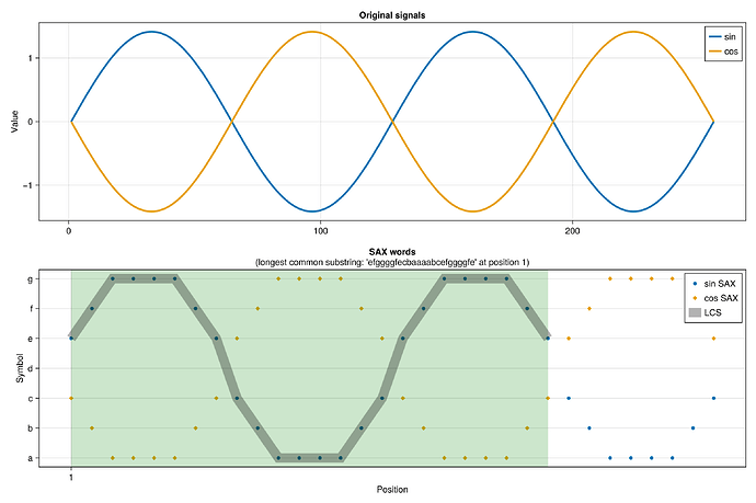
The two patterns are offset from each other by an amount that’s not necessarily a multiple of the segment size, so the elements of the resulting word don’t completely align. If on the other hand you were to deliberately make the lengths of the time series and the words all multiples of 4, like this:

signal1 = (sin.(range(0, 4Ď€, length=256)) |> x -> (x .- mean(x)) ./ std(x))
signal2 = (cos.(range(π/2, 4π+π/2, length=256)) |> x -> (x .- mean(x)) ./ std(x))  # Offset by π/2
sax = SAX(32, 7)

Then you do get practically the whole shape matching as the least common substring:

(Maybe this version would have been better for the demo. I will probably update it later.)

As for your other question, about finding the 10 longest common substrings. As a first step you could certainly use this pkg, SymbolicApproximators, to generate discretized versions of the time series at whatever resolution you feel is appropriate. (Or you could try several.) Then, although I also wrote the SuffixAutomata package that’s demonstrated here (which actually does the job of finding the lcs), I’m not sure that it’s the best choice for your task. I don’t think there’s a trivial way to find the top n common substrings.

But what you could do is something like this. Slide a window over the time series and iteratively find the lcs:

using SuffixAutomata

# two "time series" with common patterns
ts1 = "the quick brown fox jumps over the lazy dog"
ts2 = "my quick brown cat and the lazy fox went over the hill"

# build automaton from first series
sa = SuffixAutomaton(ts1)

# slide windows through second series and find matches
for window_size in [20, 15, 10], start in 1:5:length(ts2)-window_size
    window = ts2[start:start+window_size-1]
    match, pos_in_window = lcs(window, sa)
    if !isnothing(match) && length(match) >= 5
        pos_in_ts1 = findall(match, sa)[1]  # Get first occurrence in ts1
        pos_in_ts2 = start + pos_in_window - 1
        println("'$(match)' found at ts1[$pos_in_ts1] and ts2[$pos_in_ts2]")
    end
end

I’m not certain that this is the best way to go for you. But the point of this package is, it’s a way to get a discrete representation of your time series – so it opens up whole classes of algorithms that would otherwise be unavailable for continuous data. So there’s probably a better way to go than with the automata lcs that I demonstrated, I just don’t know right now what.