Very happy to announce a new package I’ve been working on to help debug ModelingToolkit.jl models. Using the power of Julia’s autodiff and the symbolics in ModelingToolkit.jl, it’s possible to estimate the error (or residual) of a model solution. Therefore it’s then possible to backout the optimal tolerance settings. Anyone who has struggled with DifferentialEquations.jl solver settings knows that sorting out a good solver choice with optimal abstol and reltol settings can be quite challenging.
For example, a gotcha that can occur is with a simple cooling model…
using ModelingToolkit
using ModelingToolkit: t_nounits as t, D_nounits as D
using OrdinaryDiffEq

T_inf=300; h=0.7; A=1; m=0.1; c_p=1.2
vars = @variables begin
    T(t)=301
end
eqs = [
    D(T) ~ (h * A) / (m * c_p) * (T_inf - T)
]
@mtkbuild sys = ODESystem(eqs, t, vars, [])
prob = ODEProblem(sys, [], (0, 10))
sol = solve(prob, Tsit5())
The temperature is expect to drop smoothly from 301K to 300K, however the plot shows us a very strange result..

What happened was simply the default tolerances don’t work well for this set of numbers. To fix the problem, we simply need to tighten the tolerance. But to what value? Should we change abstol or reltol? These values don’t have much physical meaning as it relates to the problem, therefore it’s a very difficult question to answer.
Now it’s possible to do the following…
using ModelingToolkitTolerances
resids = analysis(prob, Tsit5())
plot(resids)
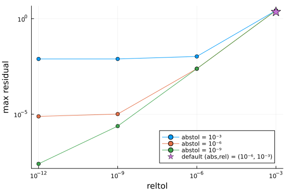
Now we can see that the default tolerance was giving a residual greater than 1. Also we can see that changing abstol does nothing in this case. Instead it’s necessary to drop reltol. Making the change gives the result we expect to see…
sol = solve(prob, Tsit5(); reltol=1e-6)
plot(sol; idxs=T)

Have a look at the README for more examples and additional utilities. Let me know what you think. Contributions and suggestions for improvement are welcome!