A super exciting update. We can now visualize any type of mesh or collection of geometries from Meshes.jl using a consistent and unified set of attributes in MeshViz.jl. Let me illustrate the features that are already available in the latest stable releases of Meshes.jl + MeshViz.jl so that you understand how general this approach is.
MeshViz.jl provides a single plot recipe called viz, which currently has the following attributes:
julia> using MeshViz

help> viz
  viz(object)

  Visualize Meshes.jl object with various options:

    •  elementcolor - color of the elements (e.g. triangles)

    •  facetcolor - color of the facets (e.g. edges)

    •  vertexcolor - color of the vertices (i.e. points)

    •  showvertices - tells whether or not to show the vertices

    •  showfacets - tells whether or not to show the facets

    •  variable - informs which variable to visualize

    •  decimation - decimation tolerance for polygons
Most often we will need to use elementcolor to color the elements of the mesh or collections of geometries. Let’s show some examples from the MeshViz.jl README:
using Meshes, MeshViz
import GLMakie

using PlyIO

function readply(fname)
  ply = load_ply(fname)
  x = ply["vertex"]["x"]
  y = ply["vertex"]["y"]
  z = ply["vertex"]["z"]
  points = Meshes.Point.(x, y, z)
  connec = [connect(Tuple(c.+1)) for c in ply["face"]["vertex_indices"]]
  SimpleMesh(points, connec)
end

mesh = readply("beethoven.ply")

viz(mesh)

mesh = readply("dragon.ply")

viz(mesh,
  showfacets=false,
  elementcolor=1:nelements(mesh),
  colormap=:Spectral
)

grid = CartesianGrid(10,10)

viz(grid)

viz(grid, elementcolor=1:nelements(grid))

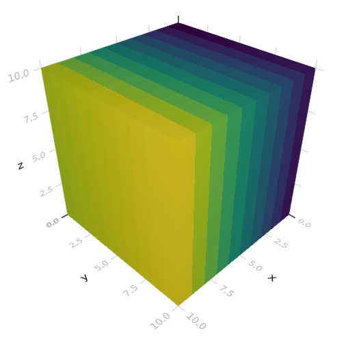
grid = CartesianGrid(10,10,10)

viz(grid)

viz(grid, elementcolor=1:nelements(grid))
We can also plot cloropleth plots at scale. This is possible because we use sophisticated Meshes.jl algorithms to simplify (or decimate) the polygonal chains before calling Makie.
To give an example, we can automatically download a very detailed map of Brazil, and plot it:
using GeoTables

# Brazil states as Meshes.jl polygons
BRA = GeoTables.gadm("BRA", children=true)

viz(BRA.geometry)

The colors are set like before using the elementcolor attribute:
viz(BRA.geometry, elementcolor=1:length(BRA.geometry))

The good news is that we can visualize any place in the world basically because we are using GADM.jl within GeoTables.jl to convert shapefiles and geopackages to Meshes.jl geometries automatically for the user. Notice how we can get the boundaries of cities inside of Rio de Janeiro:
RIO = GeoTables.gadm("BRA", "Rio de Janeiro", children=true)

viz(RIO.geometry, decimation=0.001)

The decimation tolerance controls the simplification step. The smaller the decimation the more we preserve the original boundaries of the shapes. The plan is to set this automatically in the future based on the zoom level of the visualization.
GeoStats.jl + Meshes.jl
Now the part I am really excited about ![]() We can do geostatistical estimation, simulation, learning on these domains using GeoStats.jl and produce very sophisticated geospatial workflows:
We can do geostatistical estimation, simulation, learning on these domains using GeoStats.jl and produce very sophisticated geospatial workflows:
# find row of table with Amazon geometry
ind = findfirst(==("Amazonas"), BRA.NAME_1)

# simplify geometry (thousands of vertices) before meshing
shape = simplify(BRA.geometry[ind], DouglasPeucker(0.05))

mesh = discretize(shape, FIST())

viz(mesh)

Let’s for example simulate a Gaussian field on this mesh:
using GeoStats

# ask for one realization of Gaussian variable z
problem = SimulationProblem(mesh, :z => Float64, 1)

# simple LU solver
solver = LUGS(:z => (variogram=SphericalVariogram(range=15.,),))

# simulate Gaussian field on the mesh!
sol = solve(problem, solver)

viz(sol[1], variable=:z,
  colormap = :inferno,
  showfacets=false
)

Notice that there are visualization artifacts due to the way Makie.jl interpolates the colors, and of course the mesh is also too coarse for any realistic interpolation. We are working on fixing the interpolation issue in the visualization pipeline and also working on more discretization methods that guarantee semi-regular meshes ![]()
Just for fun, let’s also create Gaussian data over a Cartesian grid (a.k.a. image data, raster data):
grid = CartesianGrid((-55.,-20.), (-45.,-10.), dims=(200,200))

problem2 = SimulationProblem(grid, :z => Float64, 1)

# for grids we can use the FFT solver
solver2 = FFTGS(:z => (variogram=SphericalVariogram(range=5.,),))

sol2 = solve(problem2, solver2)
Let’s put everything together to see how things look:
viz(BRA.geometry)

viz!(sol[1], variable=:z,
  colormap = :inferno,
  showfacets=false
)

viz!(sol2[1], variable=:z,
  colormap = :inferno,
  showfacets=false
)

If you work with geospatial data like myself, you will see the value of this unified interface. We are trying to remove all the pain people have with GIS software, and are getting very close from a very unique experience. People from other languages will wish they had something so general ![]()
This is the tip of the iceberg. I will be presenting some cool features in my JuliaCon talk next month.