# Parameter Estimation of a 3 node thermal network
**URL:** https://discourse.julialang.org/t/parameter-estimation-of-a-3-node-thermal-network/106232
**Category:** New to Julia
**Created:** [November 14, 2023, 9:00pm UTC](https://discourse.julialang.org/t/parameter-estimation-of-a-3-node-thermal-network/106232 "2023-11-14T21:00:39Z")
**Posts on this page:** 10
**Page:** 1
### Author:  [@Sooraj\_Krishnan](https://discourse.julialang.org/u/Sooraj_Krishnan)
#### Post date: [November 14, 2023, 9:00pm UTC](https://discourse.julialang.org/t/parameter-estimation-of-a-3-node-thermal-network/106232/1 "2023-11-14T21:00:39Z")
Im trying to formulate a parameter estimation problem to estimate the Resistance and Capacitance values of a 3 node thermal network. The thermal network is in the form of DAE with a mass matrix and exogenous inputs. I already have the temperature values of my 3 nodes as an interpolation function and im using it to estimate the loss of the then use Optimization.solve to solve the problem.
> using DifferentialEquations, Interpolations,
> Optimization, OptimizationPolyalgorithms, SciMLSensitivity,
> Zygote, OptimizationOptimisers, OptimizationNLopt
> using Plots
> import XLSX
> function thermal(du, u, p, t, P1, P2)
> T1, T2, T3 = u
> R\_12, R\_32, R\_35, R\_24, T4, T5 = p
> du[1] = T2/R\_12 - T1/R\_12 + P1(t);
> du[2] = T2/R\_12 + T4/R\_24 + T3/R\_32 - T2\*(1/R\_12+1/R\_24+1/R\_32);
> du[3] = T2/R\_32 + T5/R\_35 - T3\*(1/R\_32+1/R\_35) + P2(t);
> end
> p=[0.5,0.2,0.1,0.05,30,30,1000,3000,2000];
> M = [p[end-2] 0 0
> 0 p[end-1] 0
> 0 0 p[end]]
> xf = XLSX.readxlsx(“Tempdat.xlsx”)
> sh = xf[“Exp1”]
> p1 = sh[“C5:C1804”]
> p2 = sh[“D5:D1804”]
> t1 = sh[“H5:H180004”]
> t2 = sh[“I5:I180004”]
> t3 = sh[“J5:J180004”]
> d = 0.01:0.01:1800;
> t = 1:1:1800;
> tsteps = 0.1:0.1:1800
> P1=LinearInterpolation(t,vec(p1’));
> P2=LinearInterpolation(t,vec(p2’));
> T1\_s=LinearInterpolation(d,vec(t1’));
> T2\_s=LinearInterpolation(d,vec(t2’));
> T3\_s=LinearInterpolation(d,vec(t3’));
#experimental power and temperature values
> u=[20,20,20];
> tspan = (1,1800);
> f = ODEFunction(thermal, mass\_matrix = M)
> prob\_mm = ODEProblem(f, u, tspan, p)
> sol = solve(prob\_mm, Rodas5P(), saveat = 0.01, abstol=1e-8, reltol=1e-8)
> plot(sol);
> function loss(p)
> sol = solve(prob\_mm, Rodas5P(), p=p, saveat = 0.01, abstol=1e-8, reltol=1e-8)
> T1\_hat = [u[1] for u in sol.u]
> T2\_hat = [u[2] for u in sol.u]
> T3\_hat = [u[3] for u in sol.u]
>
> ```
> T1_model = T1_s(sol.t)
> T2_model = T2_s(sol.t)
> T3_model = T3_s(sol.t)
>
> loss1 = sum(abs2, T1_model .- T1_hat)
> loss2 = sum(abs2, T2_model .- T2_hat)
> loss3 = sum(abs2, T3_model .- T3_hat)
>
> loss = loss1+loss2+loss3
> return loss, sol
>
> ```
>
> end
>
> callback = function (p, l, pred)
> display(l)
>
> # plt = plot(pred)
>
> # display(plt)
>
> ```
> # Tell Optimization.solve to not halt the optimization. If return true, then
> # optimization stops.
> return false
>
> ```
>
> end
>
> #
>
> #adtype = Optimization.AutoZygote()
> #adtype = Optimization.AutoReverseDiff()
> adtype = Optimization.AutoForwardDiff()
> optf = Optimization.OptimizationFunction((x, p) → loss(x), adtype)
> optprob = Optimization.OptimizationProblem(optf, p)
>
> result\_ode = Optimization.solve(optprob, PolyOpt(), callback=callback, maxiters = 100)
I have tried with different AD solvers and different algorithms but this keeps throwing me
“ERROR: gradient of 180000-element extrapolate(scale(interpolate(::Vector{Any}, BSpline(Linear())), (0.01:0.01:1800.0,)), Throw()) with element type Float64:”
[3node\_thermal\_network.jl](https://discourse.julialang.org/uploads/short-url/lpN7cV5gpqTMIpoIWACntpnnh9b.jl) (2.2 KB)
---
### Author:  [@baggepinnen](https://discourse.julialang.org/u/baggepinnen)
#### Post date: [November 15, 2023, 5:04am UTC](https://discourse.julialang.org/t/parameter-estimation-of-a-3-node-thermal-network/106232/2 "2023-11-15T05:04:40Z")
Hello and welcome to the community 👋 Could you post the data file, such that people can run your code and reproduce the error you are seeing?
---
### Author:  [@Sooraj\_Krishnan](https://discourse.julialang.org/u/Sooraj_Krishnan)
#### Post date: [November 15, 2023, 10:36am UTC](https://discourse.julialang.org/t/parameter-estimation-of-a-3-node-thermal-network/106232/3 "2023-11-15T10:36:51Z")
Hi Fredrik,
The data file i have in a .xlsx file and i am not able to upload it, is there any other way i could possibly share the file ?
---
### Author:  [@baggepinnen](https://discourse.julialang.org/u/baggepinnen)
#### Post date: [November 15, 2023, 10:42am UTC](https://discourse.julialang.org/t/parameter-estimation-of-a-3-node-thermal-network/106232/4 "2023-11-15T10:42:04Z")
Any standard file sharing service I guess, google drive, dropbox etc.?
---
### Author:  [@Sooraj\_Krishnan](https://discourse.julialang.org/u/Sooraj_Krishnan)
#### Post date: [November 15, 2023, 10:46am UTC](https://discourse.julialang.org/t/parameter-estimation-of-a-3-node-thermal-network/106232/5 "2023-11-15T10:46:42Z")
I sharing the google drive link for the data file
> **[Loading Google Sheets](https://docs.google.com/spreadsheets/d/1NWXHJF1HQz1FWOVqr-YjPDPeXjLkQVZq/edit?usp=drive_link&ouid=103756679518539112113&rtpof=true&sd=true)**
>
> This Sheet is private
---
### Author:  [@baggepinnen](https://discourse.julialang.org/u/baggepinnen)
#### Post date: [November 15, 2023, 11:23am UTC](https://discourse.julialang.org/t/parameter-estimation-of-a-3-node-thermal-network/106232/6 "2023-11-15T11:23:35Z")
Here’s an example that uses [a simple implementation of the prediction-error method](https://www.youtube.com/watch?v=GKl8Tz9n2gs&ab_channel=JuliaHub). I call the function [`nonlinear_pem`](https://baggepinnen.github.io/ControlSystemIdentification.jl/dev/nonlinear/), even though this system is actually linear in the state and inputs.
```julia
function thermal(u, input, p, t)
P1, P2 = input
T1, T2, T3 = u
R_12, R_32, R_35, R_24, T4, T5 = p
SA[(T2/R_12 - T1/R_12 + P1) / p[end-2]
(T2/R_12 + T4/R_24 + T3/R_32 - T2*(1/R_12+1/R_24+1/R_32)) / p[end-1]
(T2/R_32 + T5/R_35 - T3*(1/R_32+1/R_35) + P2) / p[end]]
end
xf = XLSX.readxlsx("Tempdat.xlsx")
sh = xf["Exp1"]
p1 = Float64.(sh["C5:C1804"][:])
p2 = Float64.(sh["D5:D1804"][:])
t1 = Float64.(sh["H5:H180004"][:])
t2 = Float64.(sh["I5:I180004"][:])
t3 = Float64.(sh["J5:J180004"][:])
d = 0.01:0.01:1800;
t = 1:1:1800;
plot(t, u, layout=(5,1))
plot!(d, y, sp=(3:5)')
Ts = 1
t = 1:Ts:1800
## experimental power and temperature values
u = [p1 p2] # Replace with input measurement data here
y = [t1 t2 t3] # Replace with output measurement data here
d = iddata(y[1:100:end, :]', u', Ts) # Use every 100th sample of the outputs
# Initial guess
p0 = [0.5,0.2,0.1,0.05,30,30,1000,3000,2000]
u0 = SA[20.0,20,20]
R1 = 1e-4I(3) # Tuning parameters for the internal Kalman filter
R2 = 0.1I(3)
nx, nu, ny = 3, 2, 3 # Number of state variables, inputs and outputs
discrete_dynamics = SeeToDee.Rk4(thermal, Ts) # Discretize the continuous-time dynamics
measurement = (u, input, p, t) -> u # Measurement function is the identity
model = ControlSystemIdentification.nonlinear_pem(
d,
discrete_dynamics,
measurement,
p0,
u0,
R1,
R2,
nu;
optimize_x0 = false,
lower = 0.1*p0, # Constrain the search space to be within 10% of the initial guess
upper = 10*p0,
)
simplot(model, d, layout=(3, 1))
```
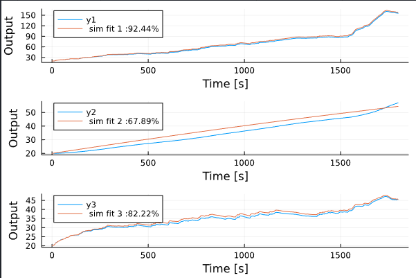
The estimated parameters are available as
```julia
julia> model.p
9-element Vector{Float64}:
0.5042616495643081
0.22669213158156562
0.10462125464969055
0.447811612771852
300.0
29.79321313071231
1006.2410623845433
30000.0
2004.2052737272784
```
The model fit is not perfect, in particular, there seem to be some problem with modeling the second output. This can be either due to missing dynamics in the model, due to the gradient-based optimizer getting stuck in a local minimum, or due to me constraining the parameters to be within 0.1-10x of the initial guess. You probably have better insight into what values are reasonable here 🙂
If the problem is due to a local minimum, you could try some form of global optimizer instead. However, this is not supported by the function `nonlinear_pem`. @SebastianM-C might have suggestions that can handle local minima better.
---
### Author:  [@baggepinnen](https://discourse.julialang.org/u/baggepinnen)
#### Post date: [November 15, 2023, 1:02pm UTC](https://discourse.julialang.org/t/parameter-estimation-of-a-3-node-thermal-network/106232/7 "2023-11-15T13:02:16Z")
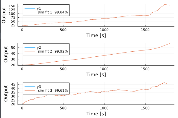
BTW, a black-box linear model of order 4 fits the data perfectly:
```julia
bbmodel, x0 = newpem(d, 4, zeroD=true, focus=:simulation)
simplot(bbmodel, dd, x0, layout = (3, 1))
```
Is the data simulated?
---
### Author:  [@Sooraj\_Krishnan](https://discourse.julialang.org/u/Sooraj_Krishnan)
#### Post date: [November 15, 2023, 3:38pm UTC](https://discourse.julialang.org/t/parameter-estimation-of-a-3-node-thermal-network/106232/10 "2023-11-15T15:38:38Z")
This is really great. Actually i have been using Matlab’s global optimization toolbox to estimate the values and been getting decent results but i haven’t tried implementing the same in Julia yet.
---
### Author:  [@Sooraj\_Krishnan](https://discourse.julialang.org/u/Sooraj_Krishnan)
#### Post date: [December 17, 2023, 1:09pm UTC](https://discourse.julialang.org/t/parameter-estimation-of-a-3-node-thermal-network/106232/11 "2023-12-17T13:09:46Z")
Hi
i have kind of modified my code to embed neural networks into my differential equation and it trains well for my training data (which is first 200sec of my simulation) but as soon as i try to extrapolate the prediction to a higher time the results don’t match. Im providing my code below, please take a look at it
using DifferentialEquations, Interpolations,Optimization, OptimizationPolyalgorithms, SciMLSensitivity,
Zygote, OptimizationOptimisers, OptimizationNLopt;
using Plots;
using OrdinaryDiffEq,DataDrivenDiffEq, ModelingToolkit, DataDrivenSparse;
using OptimizationOptimJL;
using LinearAlgebra, Statistics;
using RecursiveArrayTools,CommonSolve;
using Lux, ComponentArrays, Zygote, StableRNGs;
import XLSX
gr()
rng = StableRNG(1111)
function thermal(du, u, p\_, t)
T1, T2, T3 = u
R\_12, R\_32, R\_35, R\_24, T4, T5 = p\_
du[1] = T2/R\_12 - T1/R\_12 + P1(t);
du[2] = T1/R\_12 + T4/R\_24 + T3/R\_32 - T2\*(1/R\_12+1/R\_24+1/R\_32);
du[3] = T2/R\_32 + T5/R\_35 - T3\*(1/R\_32+1/R\_35) + P2(t);
end
p\_=[0.5,0.2,0.1,0.05,30,30,1000,3000,2000];
M = [p\_[end-2] 0 0
0 p\_[end-1] 0
0 0 p\_[end]]
xf = XLSX.readxlsx(“Tempdat.xlsx”)
sh = xf[“Exp1”]
p1 = sh[“C5:C1804”]
p2 = sh[“D5:D1804”]
t1 = sh[“H5:H180004”]
t2 = sh[“I5:I180004”]
t3 = sh[“J5:J180004”]
d = 0.01:0.01:1800;
t = 1:1:1800;
tsteps = 0.1:0.1:1800
P1=Interpolations.LinearInterpolation(t,vec(p1’));
P2=Interpolations.LinearInterpolation(t,vec(p2’));
T1\_s=Interpolations.LinearInterpolation(d,vec(t1’));
T2\_s=Interpolations.LinearInterpolation(d,vec(t2’));
T3\_s=Interpolations.LinearInterpolation(d,vec(t3’));
u=[20,20,20];
tspan = (1,200);
f = ODEFunction(thermal, mass\_matrix = M)
prob\_mm = ODEProblem(f, u, tspan, p\_)
sol = solve(prob\_mm, Rodas5P(), saveat = 0.1, abstol=1e-8, reltol=1e-8)
X = Array(sol);
t = sol.t;
plot(t, transpose(X));
rbf(x) = exp.(-(x .^ 2))
const U = Lux.Chain(Lux.Dense(2, 10, rbf), Lux.Dense(10, 10, rbf), Lux.Dense(10, 10, rbf),
Lux.Dense(10, 1))
p, st1 = Lux.setup(rng, U)
const \_st1 = st1
const V = Lux.Chain(Lux.Dense(2, 10, rbf), Lux.Dense(10, 10, rbf), Lux.Dense(10, 10, rbf),
Lux.Dense(10, 1))
q, st2 = Lux.setup(rng, V)
const \_st2 = st2
p = ComponentArray(p)
q = ComponentArray(q)
r = ComponentArray{Float64}()
r = ComponentArray(r;p)
r = ComponentArray(r;q)
p\_=[0.5,0.2,0.1,0.05,30,30,1000,3000,2000];
p\_ = ComponentArray([p\_[1], p\_[2], p\_[3], p\_[4], p\_[5], p\_[6], p\_[7], p\_[8], p\_[9]])
M = [p\_[end-2] 0 0
0 p\_[end-1] 0
0 0 p\_[end]]
# Define the hybrid model
function ude\_dynamics!(du, u, r, t)
û = U(u[1:2], r.p, \_st1)[1] # Network prediction
g = V(u[2:3], r.q, \_st2)[1]
p\_true=[0.5,0.2,0.1,0.05,30,30,1000,3000,2000];
R\_12, R\_32, R\_35, R\_24, T4, T5 = p\_true
du[1] = û[1] + P1(t) ;
du[2] = -û[1] + (T4-u[2])/R\_24 + g[1];
du[3] = -g[1] + (T5-u[3])/R\_35 + P2(t);
end
ude\_dynamics = ODEFunction(ude\_dynamics!, mass\_matrix = M)
#nn\_dynamics(du, u, p, t) = ude\_dynamics(du, u, p, t)
prob\_nn = ODEProblem(ude\_dynamics, X[:, 1], tspan, r)
function predict(θ, x = X[:, 1], T = t)
```
#_prob = remake(prob_nn, u0 = x, tspan = (T[1], T[end]), p=θ)
Array(solve(prob_nn, Rodas5P(), p=θ, saveat = 0.1,
abstol = 1e-8, reltol = 1e-8,
sensealg=QuadratureAdjoint(autojacvec=ReverseDiffVJP(true))))
```
end
function loss(θ)
X̂ = predict(θ)
mean(abs2, X .- X̂)
end
losses = Float64
callback = function (r, l)
push!(losses, l)
if length(losses) % 50 == 0
println(“Current loss after (length(losses)) iterations: (losses[end])”)
end
return false
end
adtype = Optimization.AutoZygote()
optf = Optimization.OptimizationFunction((x, r) → loss(x), adtype)
optprob = Optimization.OptimizationProblem(optf,r)
res1 = Optimization.solve(optprob, ADAM(), callback = callback, maxiters = 1000)
println(“Training loss after (length(losses)) iterations: (losses[end])”)
optprob2 = Optimization.OptimizationProblem(optf, res1.u)
res2 = Optimization.solve(optprob2, Optim.LBFGS(), callback = callback, maxiters = 5000)
println(“Final training loss after (length(losses)) iterations: (losses[end])”)
# Rename the best candidate
p\_trained = res2.u
pl\_losses = plot(1:1000, losses[1:1000], yaxis = :log10, xaxis = :log10,
xlabel = “Iterations”, ylabel = “Loss”, label = “ADAM”, color = :blue)
plot!(1001:length(losses), losses[1001:end], yaxis = :log10, xaxis = :log10,
xlabel = “Iterations”, ylabel = “Loss”, label = “BFGS”, color = :red)
#ts = first(sol.t):(mean(diff(sol.t)) / 2):last(sol.t)
X̂ = predict(p\_trained, X[:, 1], t)
# Trained on noisy data vs real solution
pl\_trajectory = plot(t, transpose(X̂), xlabel = “t”, ylabel = “T1(t), T2(t),T3(t)”,
label = [“UDE Approximation” nothing])
---
### Author:  [@Sooraj\_Krishnan](https://discourse.julialang.org/u/Sooraj_Krishnan)
#### Post date: [December 17, 2023, 1:14pm UTC](https://discourse.julialang.org/t/parameter-estimation-of-a-3-node-thermal-network/106232/12 "2023-12-17T13:14:39Z")
I have built upon the example that was provided in documentation [Automatically Discover Missing Physics by Embedding Machine Learning into Differential Equations · Overview of Julia's SciML](https://docs.sciml.ai/Overview/stable/showcase/missing_physics/#Symbolic-regression-via-sparse-regression-(SINDy-based))
i have a different variation of code where i tried to learn one part of each of my 3 equations using one neural network but that too didn’t work.
rbf(x) = exp.(-(x .^ 2))
const U = Lux.Chain(Lux.Dense(3, 5, rbf), Lux.Dense(5, 5, rbf), Lux.Dense(5, 5, rbf),
Lux.Dense(5, 3))
p\_, st = Lux.setup(rng, U)
const \_st = st
function ude\_dynamics!(du, u, p\_, t, p\_true)
û = U(u, p\_, \_st)[1] # Network prediction
T1, T2, T3 = u
R\_12, R\_32, R\_35, R\_24, T4, T5 = p\_true
du[1] = T2/R\_12 - û[1] + P1(t);
du[2] = T2/R\_12 + T4/R\_24 + T3/R\_32 - û[2];
du[3] = T2/R\_32 + T5/R\_35 - û[3] + P2(t);
end
Im not able to understand why my implementation is not working, is it because i have a mass matrix and exogenous inputs involved ? if so how can i embed neural networks into ODE problems with both exogenous inputs and a mass matrix so that i can learn certain parts of my differential equation ??